Climate Coupling and Hidden Economic Costs
by Daniel Brouse
March 25, 2026
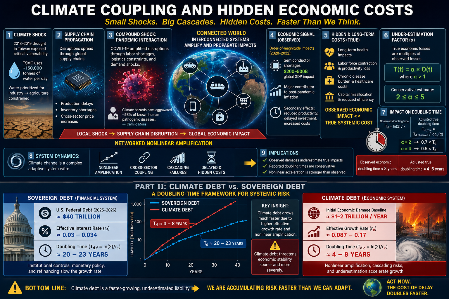
The true economic cost of climate change is amplified through interconnected system dynamics, where localized climate shocks propagate through global supply chains and interact with concurrent systemic risks. A prominent example is the coupling of drought, semiconductor production, and the COVID-19 pandemic.
1. Climate Shock: Water Scarcity and Semiconductor Production
The 2018–2019 drought in Taiwan exposed the sensitivity of critical infrastructure to hydroclimatic variability. Semiconductor manufacturing is highly water-intensive; TSMC consumes on the order of 150,000 tonnes of water per day. During drought conditions, water allocation was prioritized toward industrial production, constraining agricultural systems while exposing a critical vulnerability in global semiconductor supply chains.
2. Supply Chain Propagation
Semiconductors are foundational inputs across multiple sectors, including automotive manufacturing, consumer electronics, telecommunications, and industrial systems. Disruptions propagated globally, producing:
- Production delays
- Inventory shortages
- Cross-sector price increases
This propagation can be generalized as:
Local Shock -> Supply Chain Disruption -> Global Economic Impact
This reflects networked nonlinear amplification, where tightly coupled systems transmit localized perturbations across global scales.
3. Compound Shock: Pandemic Interaction
The emergence of COVID-19 amplified these disruptions through labor shortages, logistical constraints, and demand shocks.
Research by Camilo Mora indicates that climate hazards have aggravated approximately 58% of known human pathogenic diseases, highlighting that climate change acts as a systemic risk multiplier across environmental, biological, and economic domains.
4. Quantifying the Economic Signal
Although precise attribution remains complex, multiple estimates provide order-of-magnitude bounds:
- Semiconductor shortages (2020–2022): ~$200–500 billion global GDP impact
- Supply chain disruptions: major contributor to post-pandemic inflation
- Secondary effects: reduced productivity, delayed investment, increased costs
These represent propagated economic losses, not direct climate damages.
5. Hidden and Long-Term Costs
The full cost extends beyond observed economic signals:
- Long-term health impacts (e.g., persistent multi-system effects)
- Labor force contraction and productivity loss
- Chronic disease burden and healthcare costs
- Capital misallocation and reduced efficiency
This implies:
Observed Economic Impact << True Systemic Cost
6. Quantifying Underestimation
Define:
- O(t) = observed economic losses
- T(t) = true economic losses
- alpha = underestimation factor
Then:
T(t) = alpha * O(t), where alpha > 1
Based on integrated assessment models and disaster economics literature, a conservative estimate is:
2 <= alpha <= 5
This implies that true economic impacts may be 2x to 5x larger than observed values.
7. Impact on Doubling Time
Because growth is exponential, underestimation compresses the effective doubling time.
Observed doubling time:
T_d_observed = ln(2) / k
True doubling time:
T_d_true = ln(2) / (k + ln(alpha)/delta_t)
Approximation:
T_d_true ≈ T_d_observed / log2(alpha)
Examples:
- If alpha = 2 → T_d_true ≈ 0.7 * T_d_observed
- If alpha = 4 → T_d_true ≈ 0.5 * T_d_observed
Thus:
- Observed economic doubling time ≈ 8 years
- Adjusted true doubling time ≈ 4–6 years
8. System Dynamics Interpretation
This case demonstrates that climate change behaves as a complex adaptive system characterized by:
- Nonlinear amplification
- Cross-sector coupling
- Cascading failures
- Delayed and hidden costs
Small perturbations (e.g., drought) can produce disproportionately large global outcomes, especially when interacting with concurrent shocks.
9. Implications
The presence of hidden and amplified costs implies:
- Observed damages underestimate true impacts
- Reported doubling times are conservative
- Nonlinear acceleration is stronger than observed
This reinforces the conclusion that climate impacts are accelerating through higher-order dynamics (including positive third derivatives) and cascading feedbacks consistent with nonlinear instability.
Part II – Climate Debt vs. Sovereign Debt: A Doubling-Time Framework for Systemic Risk
Abstract
This section introduces a comparative framework between sovereign financial debt and an implied “climate debt,” defined as the cumulative and compounding economic costs of climate change. By modeling both systems as exponential processes, we demonstrate that climate-related liabilities exhibit significantly shorter doubling times due to higher effective growth rates. This divergence provides further evidence of nonlinear amplification and higher-order dynamics in climate–economic systems.
1. Conceptual Framework
Sovereign debt and climate-related economic damages can both be represented as compounding liabilities:
D(t) = D_0 * e^(r * t)
Where:
D(t)= total liability at timetD_0= initial valuer= effective growth ratet= time
The doubling time is:
T_d = ln(2) / r
This formulation allows direct comparison between financial and climate-driven systems.
2. Financial Debt Baseline
As of 2025–2026, total U.S. federal debt is approximately:
D_f ≈ $40 trillion
The effective weighted-average interest rate on this debt is approximately:
r_f ≈ 0.03–0.034
This yields a doubling time:
T_d_f = ln(2) / r_f ≈ 20–23 years
This relatively long doubling time reflects institutional controls, monetary policy intervention, and refinancing structures (U.S. Department of the Treasury; Congressional Budget Office).
3. Climate Debt Approximation
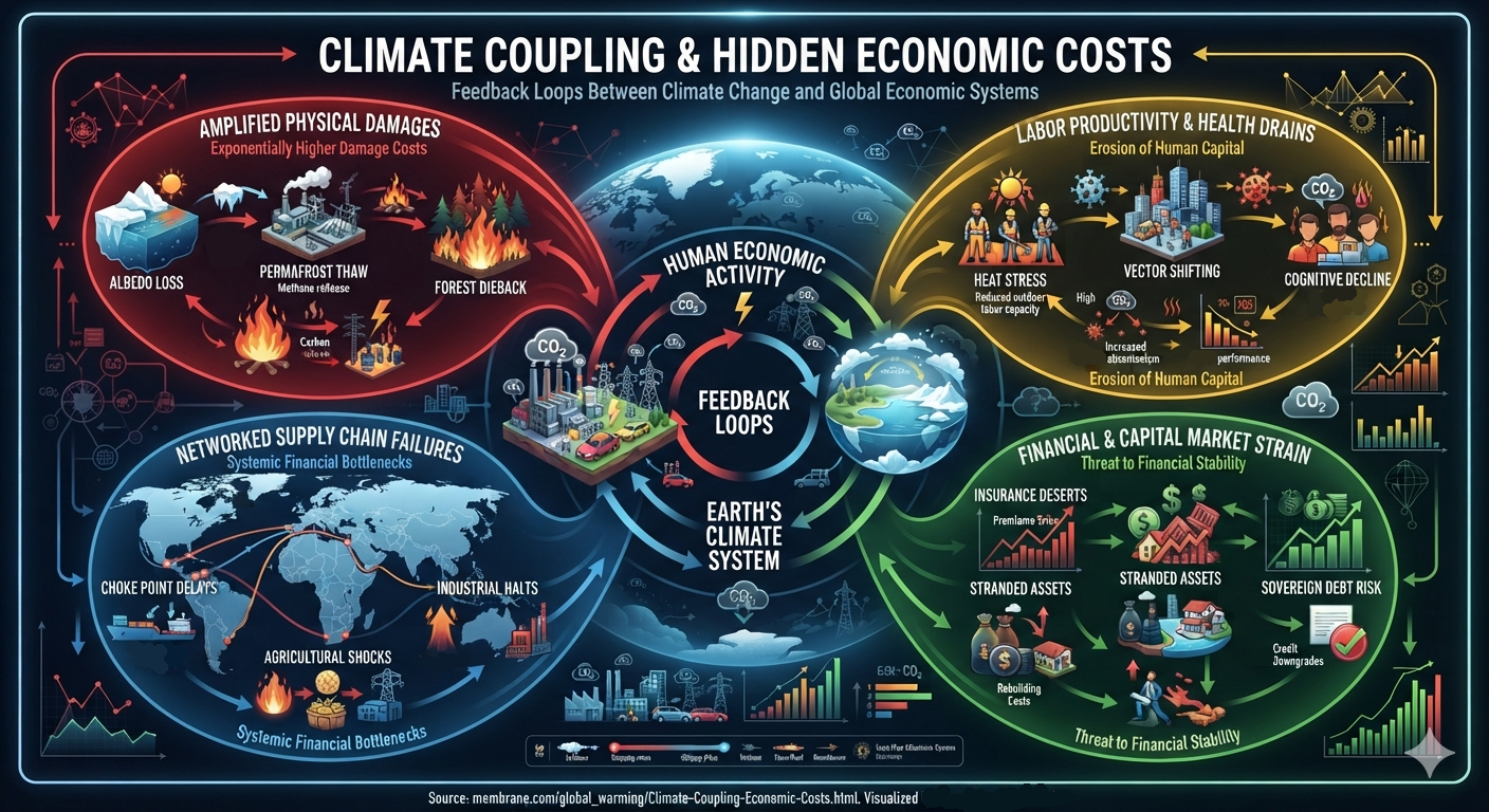
We define climate debt as the total economic liability arising from:
- Physical damages (storms, floods, wildfires)
- Infrastructure degradation
- Health impacts
- Supply chain disruptions
- Long-term productivity loss
Given substantial underestimation in reported damages, we assume a conservative baseline:
D_c ≈ $40 trillion
This is consistent with integrated assessments suggesting that climate damages may reach several multiples of annual global GDP under high-emissions scenarios (Intergovernmental Panel on Climate Change; Swiss Re).
4. Effective Growth Rate of Climate Damages
Empirical observations indicate that climate-related economic damages are growing at an accelerated rate. Based on observed doubling times of billion-dollar disasters (~8 years), we estimate:
r_c ≈ 0.10–0.15
This reflects:
- Nonlinear amplification
- Increasing exposure
- Feedback-driven escalation
(National Oceanic and Atmospheric Administration; Intergovernmental Panel on Climate Change)
5. Doubling-Time Comparison
Applying the exponential model:
Financial Debt:
T_d_f ≈ 20–23 years
Climate Debt:
T_d_c (10%) ≈ 6.9 years
T_d_c (15%) ≈ 4.6 years
This yields:
T_d_c << T_d_f
or equivalently:
r_c >> r_f
6. Divergence Over Time
Over a 20-year horizon:
Financial Debt:
D_f(20) ≈ 40T * e^(0.032 * 20) ≈ $75–80 trillion
Climate Debt:
At 10%:
D_c(20) ≈ 40T * e^(2.0) ≈ $296 trillion
At 15%:
D_c(20) ≈ 40T * e^(3.0) ≈ $804 trillion
Thus:
Climate Debt / Financial Debt ≈ 4× to 10× (within ~20 years)
7. Nonlinear Amplification Mechanisms
The divergence between financial and climate debt is driven by structural differences:
Financial Debt
- Policy-constrained
- Adjustable via interest rates and taxation
- Governed by institutional frameworks
Climate Debt
- Driven by physical processes
- Amplified by feedback loops
- Coupled across environmental and economic systems
These amplification pathways include:
- Topographic amplification of flooding
- Increasing infrastructure exposure
- Intensification of extreme events
- Insurance withdrawal and financial contagion
(Marshall Burke et al., 2015; Solomon Hsiang et al., 2017)
8. Higher-Order Dynamics and Instability
The climate system exhibits higher-order dynamics:
dD/dt > 0
d²D/dt² > 0
d³D/dt³ > 0
Where:
- First derivative: impacts increasing
- Second derivative: acceleration increasing
- Third derivative: acceleration of acceleration increasing
This third-derivative behavior (“jerk”) indicates a system approaching nonlinear instability, where growth rates themselves are increasing over time.
9. Implications
The key implication is that climate debt behaves as a high-interest compounding liability:
Climate Debt behaves like a liability with 3–5× faster doubling time than sovereign debt.
Because:
dD_c/dt >> dD_f/dt
It follows that:
Total System Risk → Dominated by Climate Debt over time
10. Conclusion
This analysis demonstrates that:
- Financial debt grows at a relatively modest rate (~3%), with doubling times of ~20–23 years.
- Climate-related economic damages grow substantially faster (~10–15%), with doubling times of ~5–7 years.
- This divergence leads to a rapid expansion of climate liabilities relative to sovereign debt.
- The presence of higher-order dynamics (
d³D/dt³ > 0) suggests that current estimates are likely conservative. - Within one to two decades, climate debt may exceed financial debt by an order of magnitude, representing a dominant source of systemic risk.
These findings reinforce the broader conclusion that climate change is not merely an environmental issue, but a rapidly accelerating financial liability governed by nonlinear dynamics. More importantly, these systems are interconnected through reinforcing feedback loops. As climate-related damages increase alongside sovereign debt burdens, upward pressure on effective interest rates is likely to emerge, driven by heightened risk, fiscal strain, and capital reallocation. This dynamic compounds long-term liabilities, increasing the probability of unsustainable debt trajectories for future generations. If left unmitigated, such coupled dynamics may accelerate systemic financial instability and elevate the risk of broader economic disruption.
References
- A Unified Energetics Framework for Accelerating Climate Change: From Radiative Forcing to Drag Physics -- Brouse and Mukherjee (2026)
- Emergent Climate Dynamics: The Nonlinear Acceleration of Climate Impacts -- Brouse and Mukherjee (2026)
- The Third Derivative and Climate Acceleration: Why Change Is Increasing Faster Over Time -- Brouse (2026)
- Intergovernmental Panel on Climate Change (2023). Sixth Assessment Report
- Camilo Mora et al. (2022). Climate hazards and infectious disease
- Swiss Re (2022). Sigma Report
- Daron Acemoglu et al. (2012). Network effects in macroeconomics
- Marshall Burke et al. (2015). Climate impacts on economic output
- U.S. Department of the Treasury
- Congressional Budget Office
- Intergovernmental Panel on Climate Change
- National Oceanic and Atmospheric Administration
- Swiss Re
- Solomon Hsiang et al. (2017)
A subsection of:
How Not to Be a Jerk: Third Derivatives and the Singularity of Climate Change